
OlmoEarth v1.1: A More Efficient Family of Earth Observation Models
Team post, published on May 19, 2026
- Increasing efficiency by decreasing sequence lengths
- Designing the token
- For developers
- For researchers
- Get started
🧠 Models: https://huggingface.co/collections/allenai/olmoearth | 📄 Technical report: https://allenai.org/papers/olmoearth_v1_1 | 💻 Code: https://github.com/allenai/olmoearth_pretrain
We released OlmoEarth (v1) in November 2025. Since then, partners have applied it to a wide range of tasks, from tracking mangrove change and classifying the drivers of forest loss to producing country-scale crop type maps in just days, and scaling deployments to national, continental, and even global levels. Each release brings us closer to our mission: bringing state-of-the-art AI to the organizations and communities working to protect people and the planet.
When OlmoEarth processes satellite imagery and makes predictions across tens of thousands to hundreds of thousands of square kilometers, efficiency determines what is possible. Across the entire lifecycle of running OlmoEarth — data export, preprocessing, inference, and postprocessing — compute costs are by far the biggest expense. A more efficient model means we can support more partners on the OlmoEarth Platform, and it also means anyone running OlmoEarth on their own can use the technology faster and at lower cost.
That is why we built OlmoEarth v1.1: a new family of models that preserves OlmoEarth v1 performance across a range of research benchmarks and tasks we developed with partners, while reducing compute cost by up to 3x.
Increasing efficiency by decreasing sequence lengths
OlmoEarth models are transformer-based, and transformers are one of the dominant architectures in machine learning today. To process remote sensing data, we first convert it into a sequence of tokens that the model can consume.
There are two important levers that affect the efficiency of transformer models: model size — which is why we release a family of models, so users can choose the right size for their compute budget — and token sequence length. Compute cost grows quadratically with token sequence length, so even small reductions can significantly lower the cost of running a model.
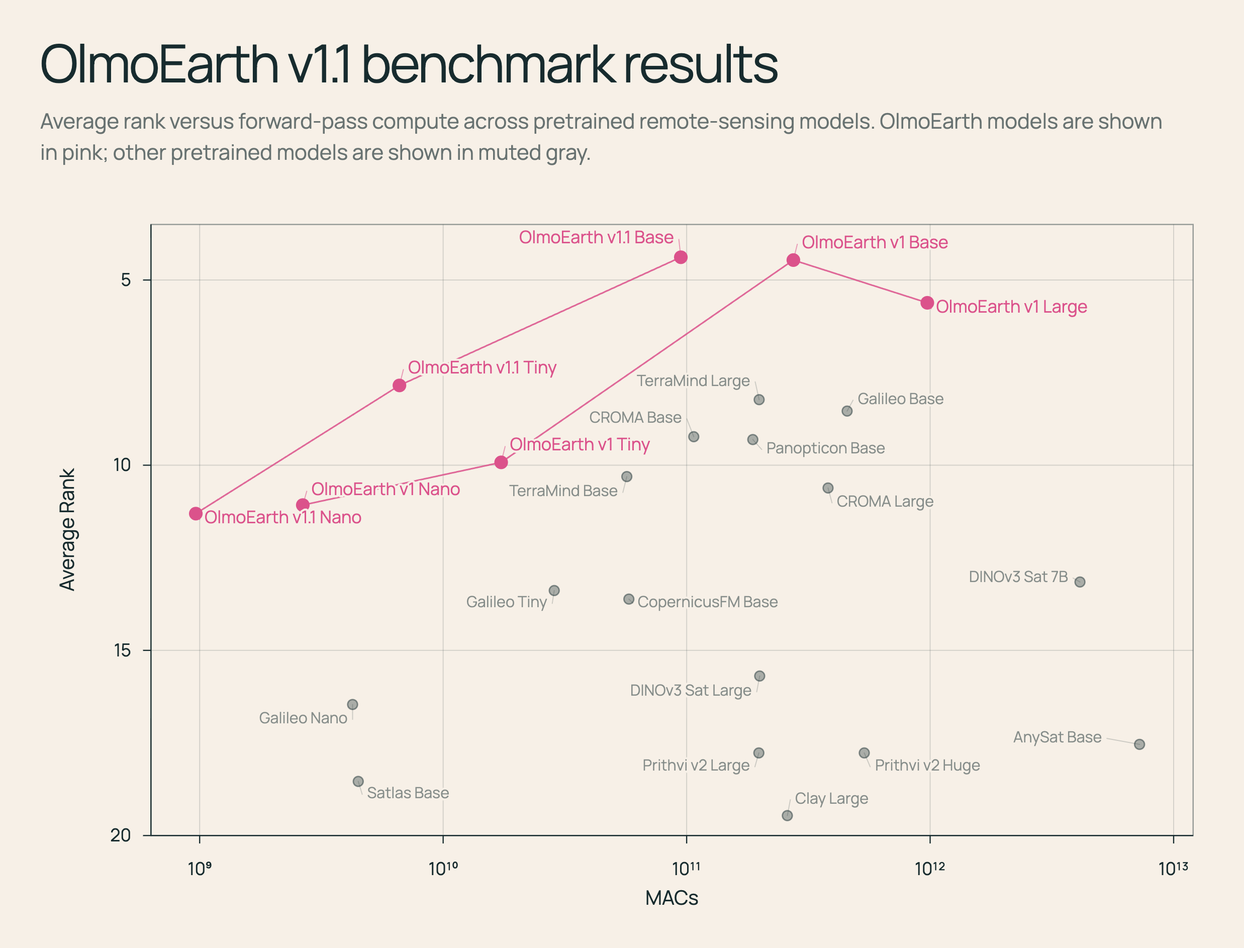
MACs (multiply-accumulate operations) are used to estimate the compute required for a single model forward pass; lower MACs generally mean lower inference cost and faster speed. The y-axis is inverted because lower average rank is better. Labels show the model family and size. All plotted points use the MAC/rank values shown in the figure.
Designing the token
This raises an important question for transformer-based remote sensing models: what should a token represent?
Consider Sentinel-2 imagery, one of the common modalities we work with. A Sentinel-2 input is a tensor with height and width (H, W, representing pixels in latitude and longitude), a temporal dimension T, and 12 Sentinel-2 channels ([H, W, T, D=12]).
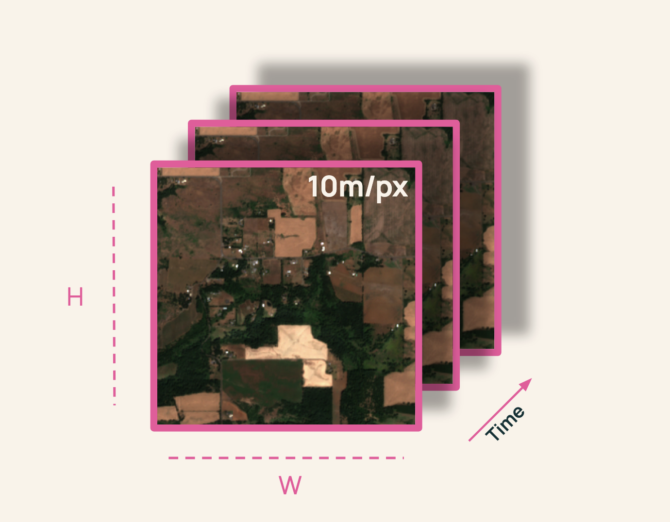
Today, we split the data into resolution-based patches. Concretely, this means we choose a spatial patch size p and then divide the entire Sentinel-2 image into p x p patches:
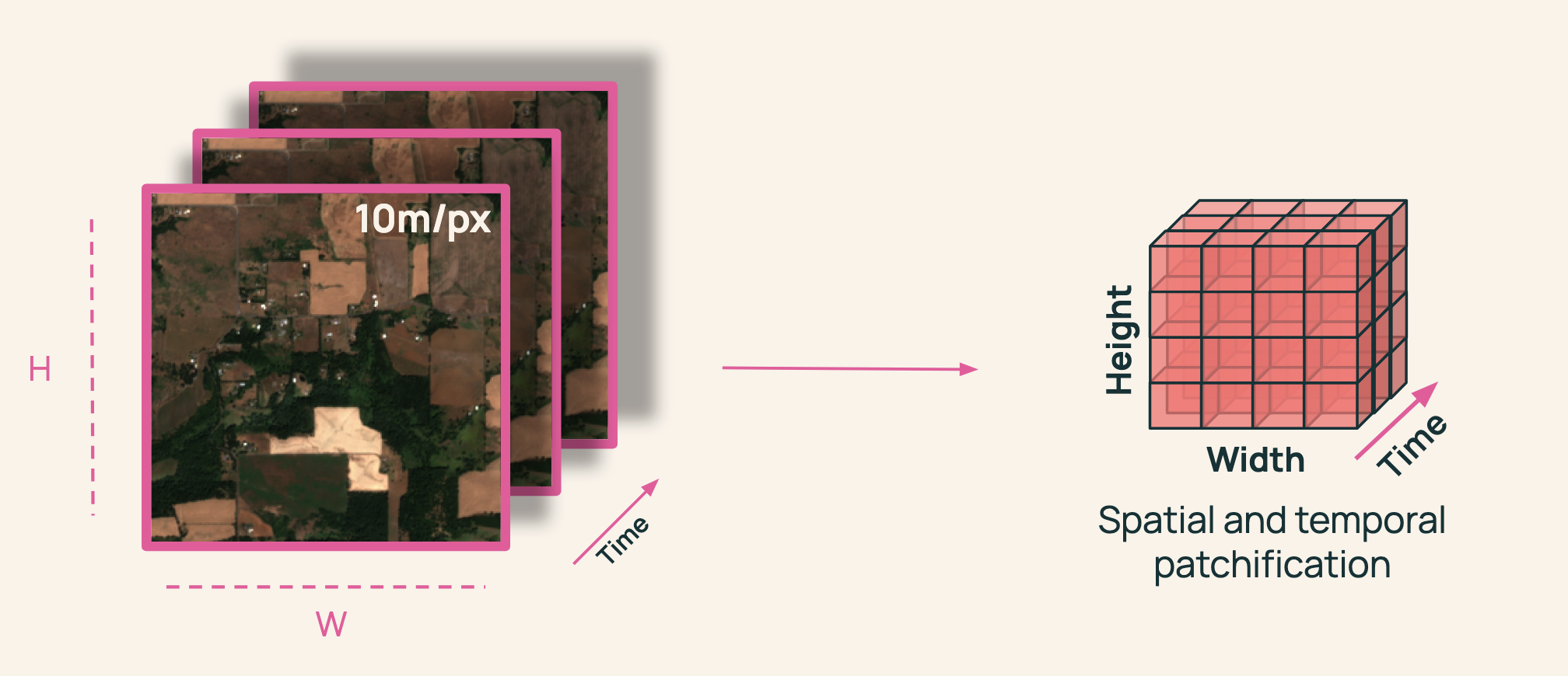
For each patch, we create a token at each time step and for each resolution. So a Sentinel-2 input with 2 time steps yields 6 tokens per patch (2 time steps × 3 resolutions, 10m, 20m, and 60m).
In total, a Sentinel-2 input of [H, W, T, D=12] will produce H/p × W/p × T × 3 tokens.
Using a unique token for each resolution is a common technique for working with Sentinel-2 data — Galileo and [SatMAE](https://arx